A Quick Look at B-cos Nets' Adversarial Robustness

Update-25-11-2023: Added B-cos ResNet-50 (trained with the default hyperparameters).

Update-23-11-2023: As noted by Navdeeppal Singh, the comparison between ResNet-50 and B-cos ResNet-56 is not fair, due to architectural, augmentation, and hyperparameter differences. A previous version of this post claimed reproducing some results from [3], which was inaccurate. The post was edited to reflect those notes.

Table of Contents

1. Introduction
2. Training B-cos Nets
3. Quantitative Results
4. Qualitative Results
5. Conclusion
6. References

1. Introduction

Inherently interpretable models are a class of models that prioritize interpretability during the optimization process, contrasting with post-hoc interpretability methods that address interpretability after training is complete. B-cos models represent an example of inherently interpretable models. For a high-level overview, refer to this post, talk, and presentation. For a more in-depth treatment, consult the papers on CoDA Nets [1], B-cos Nets [2], and B-cos ViTs [3].

In this post, I attempt to train two B-cos models on CIFAR10, namely B-cos ResNet-56 and B-cos ResNet-50 (Section 2), evaluate their adversarial robustness, and compare it to naturally and adversarially trained networks, both quantitatively (Section 3) and qualitatively (Section 4). The code used to generate the results presented in this post can be found in this notebook or .

2. Training B-cos Nets

Executing the published code was straightforward, except for the need to modify train-requirements.txt to specify PyTorch Lightning’s version to be pytorch-lightning==1.9.0, as Lighting versions from 2.0.0 upwards were incompatible [fixed]. Specifically, I trained a Bcos-ResNet-56 model on CIFAR10 by running the command:

python train.py \
     --dataset CIFAR10 \
     --base_network norm_ablations_final \
     --experiment_name resnet_56-nomaxout

and a B-cos ResNet-50 by running the command:

python train.py \
     --dataset CIFAR10 \
     --base_network large_nets \
     --experiment_name resnet_50

The obtained test accuracies were 88.06% with 100 epochs and 87.42% with 90 epochs, respectively. The performance could be improved with more hyperparameter tuning, especially for the B-cos ResNet-50 since it was overfitting. Figure 1 depicts the top-1 and top-5 accuracies on the train and evaluation sets throughout the epochs of training. The trained checkpoint weights can be downloaded from this repository.

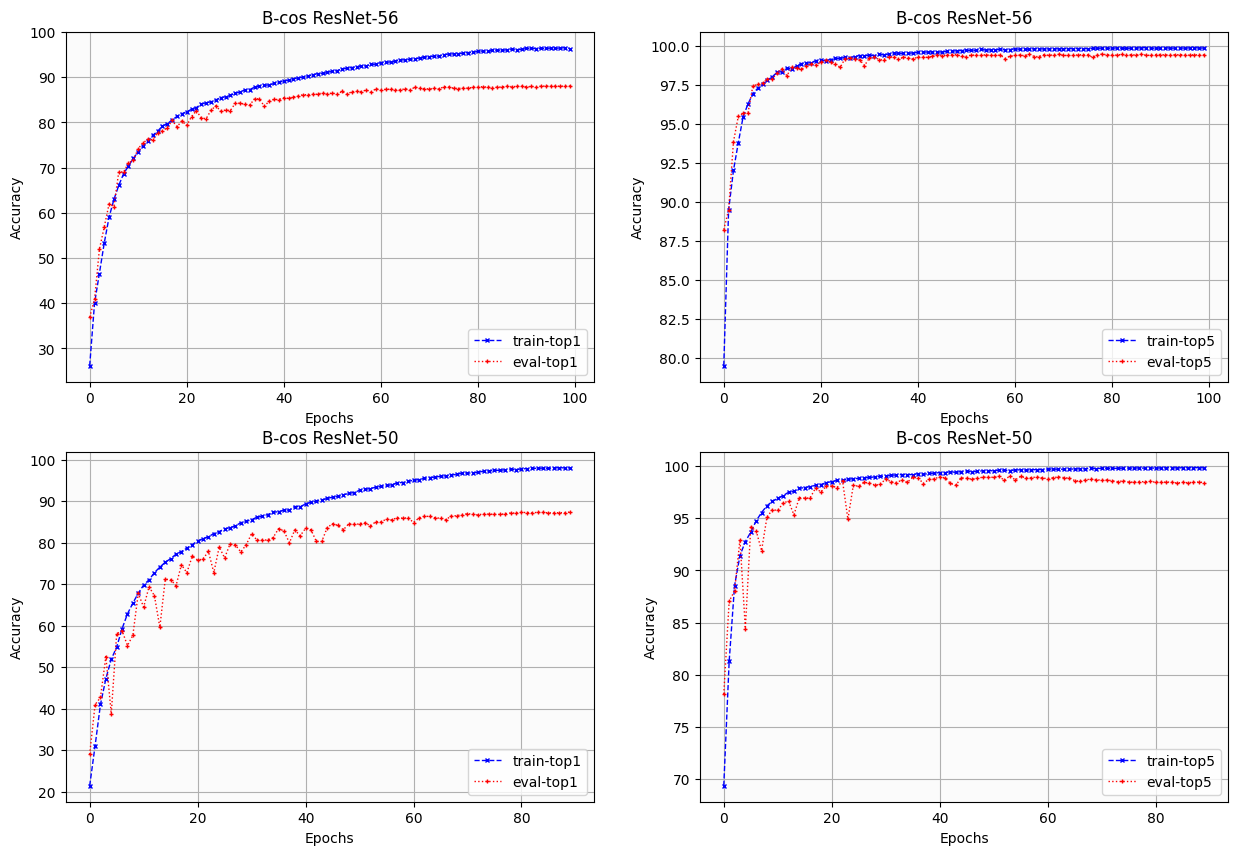
Fig.1: Evolution of top-1 and top-5 accuracies on train and evaluation sets during training.

3. Quantitative Results

To evaluate the adversarial robustness of the trained B-cos models, I utilized the Robustness library [4]. The library provides access to naturally and adversarially pretrained ResNet-50 models (link to pretrained models). In addition, this library makes it easy to attack a custom loss function, which comes in handy in this case due to the Binary Cross-Entropy loss function employed during the B-cos models training process.

Tables 1 and 2 present the accuracies of the models against \(\ell_\infty\) and \(\ell_2\) PGD attacks, respectively. Each cell corresponds to the accuracy achieved against (20-step/100-step) PGD attacks with a step size of 2.5 * ε-test / num_steps, following [4]. The Adv-ResNet-50 model in Table 1 is an \(\ell_\infty\) adversarially trained model with \(\epsilon=8/255\) (model checkpoint), while in Table 2 it is an \(\ell_2\) adversarially trained model with \(\epsilon=0.5\) (model checkpoint).

It is important to note that the results presented herein should be interpreted with caution due to the disparity in architecture and data augmentation pipelines employed for the B-cos ResNet-56 model and the provided ResNet-50 models. In addition, due to computational limitations, no detailed hyperparameter tuning was done for the B-cos ResNet-50.

Table 1	Standard Accuracy	\(\epsilon=8/255\)	\(\epsilon=16/255\)
ResNet-50	95.25%	0.0% / 0.0%	0.0% / 0.0%
Adv-ResNet-50	87.03%	53.49% / 53.29%	18.13% / 17.62%
Bcos-ResNet-56	88.06%	0.03% / 0.03%	0.0% / 0.0%
Bcos-ResNet-50	87.42%	19.79% / 19.10%	8.33% / 7.68%

Table 1: CIFAR-10 test accuracy against PGD \(\ell_\infty\) attacks.

Table 2	Standard Accuracy	\(\epsilon=0.25\)	\(\epsilon=0.5\)	\(\epsilon=1.0\)	\(\epsilon=2.0\)
ResNet-50	95.25%	8.66% / 7.34%	0.28% / 0.14%	0.0% / 0.0%	0.0% / 0.0%
Adv-ResNet-50	90.83%	82.34% / 82.31%	70.17% / 70.11%	40.47% / 40.22%	5.23% / 4.97%
Bcos-ResNet-56	88.06%	35.06% / 34.75%	13.64% / 13.20%	9.02% / 8.91%	0.0% / 0.0%
Bcos-ResNet-50	87.42%	65.64% / 65.71%	50.19% / 49.96%	33.16% / 32.04%	15.01% / 14.57%

Table 2: CIFAR-10 test accuracy against PGD \(\ell_2\) attacks.

In contrast to naturally trained models, B-cos networks exhibited inherent robustness, particularly against \(\ell_2\) attacks, outperforming even adversarially trained models at the largest epsilon tested. These findings provide evidence that inherently interpretable models represent a promising direction for both interpretability and robustness.

4. Qualitative Results

Driven by curiosity, I wanted to investigate how B-cos models’ explanations and contribution maps change when attacked. Figures 2, 3, 4, and 5 illustrate a set of example inputs from the CIFAR10 test set, along with their attacked counterparts. These figures showcase the induced adversarial noise, the explanations and contribution maps generated by the B-cos models for both the normal and attacked inputs, and their corresponding differences.

Note that the difference images are per-row normalized to be between 0 and 1. Therefore, care should be taken when trying to interpret these images (refer to the associated colorbars for magnitude reference).

4.1 B-cos ResNet-56

Figures 2 and 3 depict the results for B-cos ResNet-56 with \(\ell_2\) and \(\ell_\infty\) attacks, respectively.

In the second column (frog) of Figure 2 for example, the adversarial noise exhibits a grid-like pattern reminiscent of a truck’s front grille. This pattern is reflected in the corresponding attacked contribution map and may explain the model’s misclassification of the input as a truck.

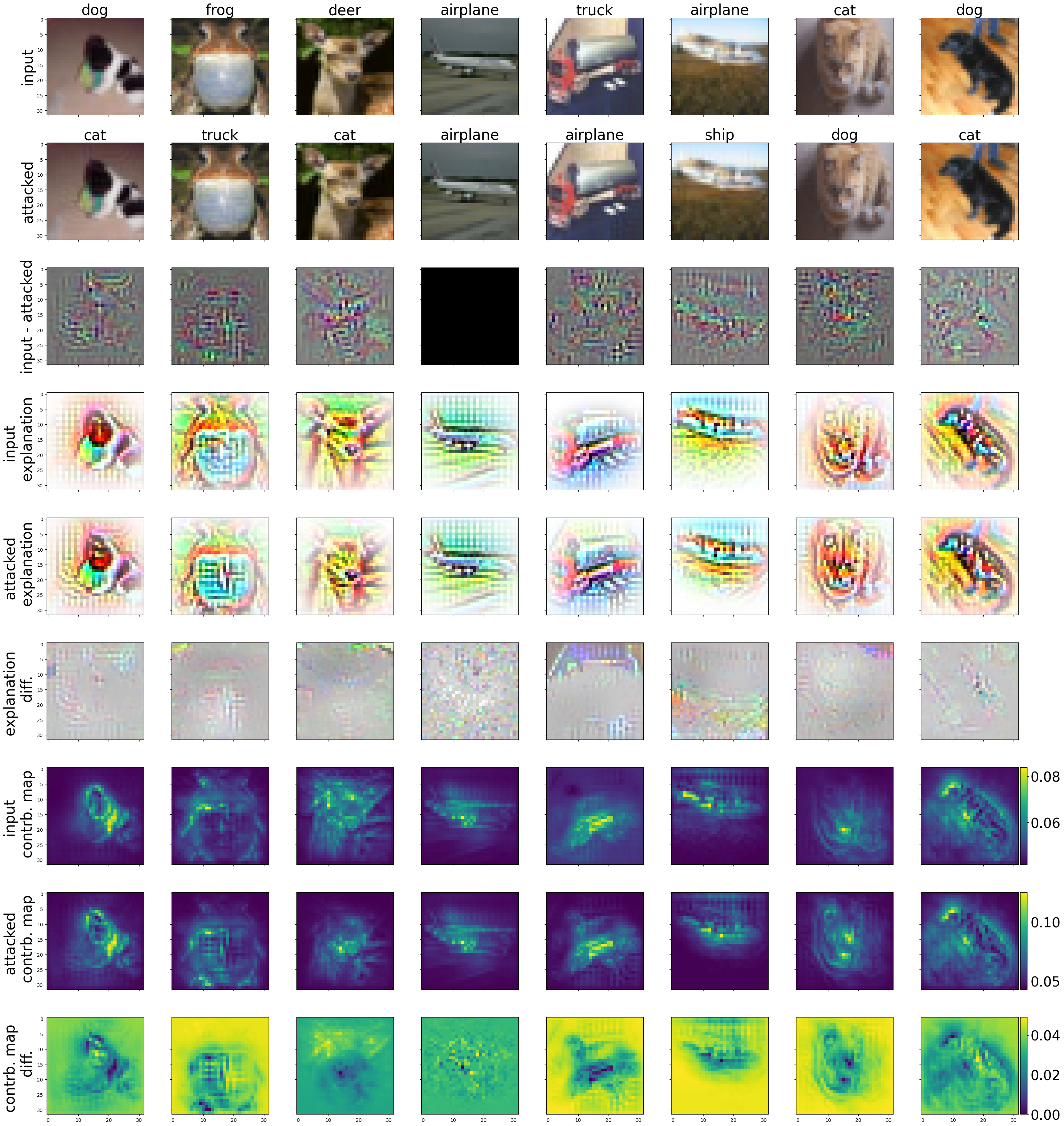
Fig. 2: Example of inputs to B-cos ResNet-56 attacked with \({\ell_2}\) PGD with 100 steps and \({\epsilon=0.5}\).

Similarly, in Figure 3, column 7 (cat) is misclassified as a dog. Examining its contribution map difference, it is plausible to interpret it as a dog’s head rather than that of a cat.

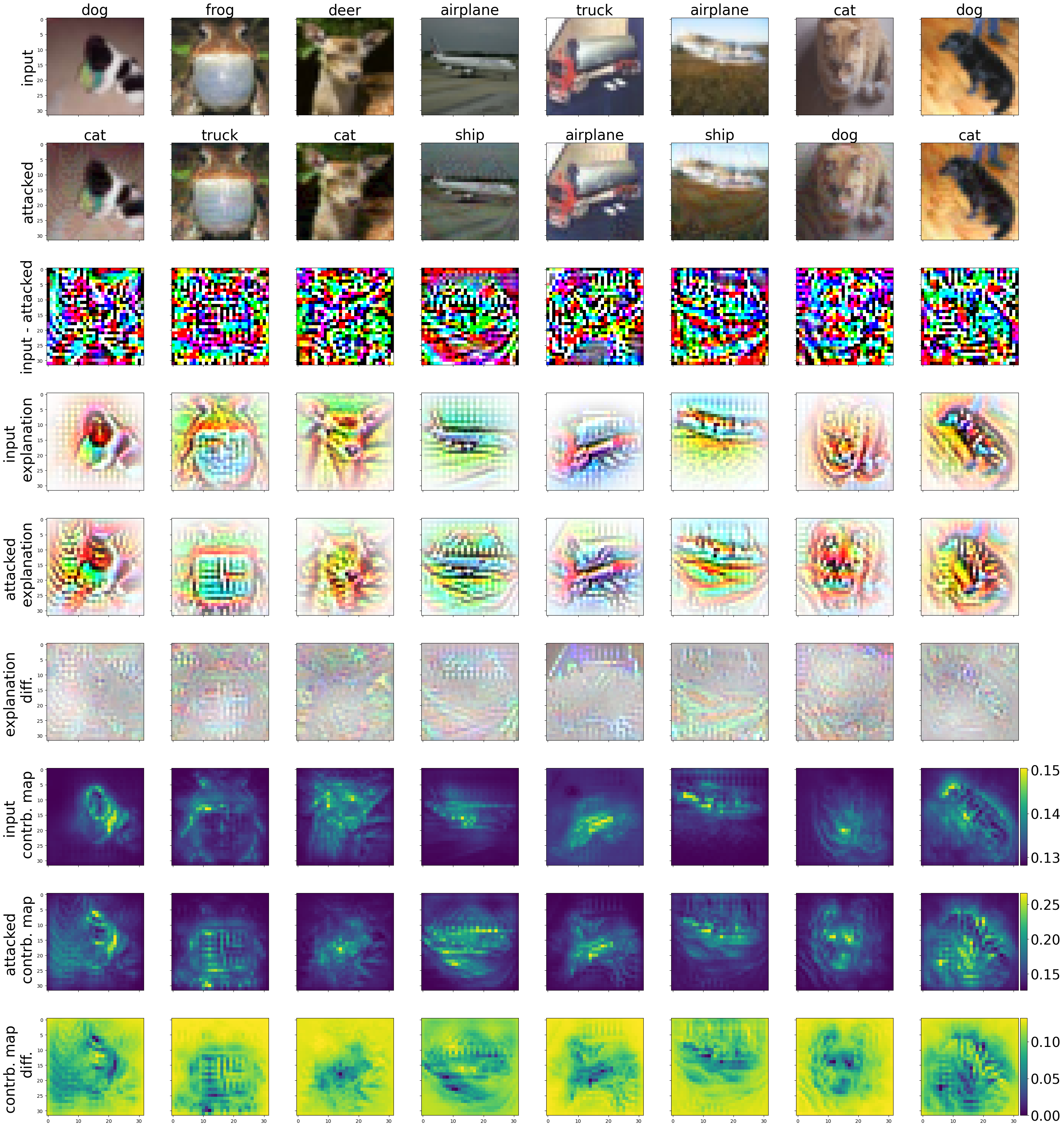
Fig. 3: Example of inputs to B-cos ResNet-56 attacked with \({\ell_\infty}\) PGD with 100 steps and \({\epsilon=8/255}\).

4.2 B-cos ResNet-50

Figures 4 and 5 depict the results for B-cos ResNet-50 with \(\ell_2\) and \(\ell_\infty\) attacks, respectively. We can see that the explanations for this model are less detailed and input-aligned than the ones for the B-cos ResNet-56 shown above. In addition, B-cos ResNet-50’s contribution maps show a grid-like structure, which was not present for B-cos ResNet-56. These artifacts could be attributed to both the architectural differences between the two models, as well as the lack of fine-tuning done for the presented B-cos ResNet-50.

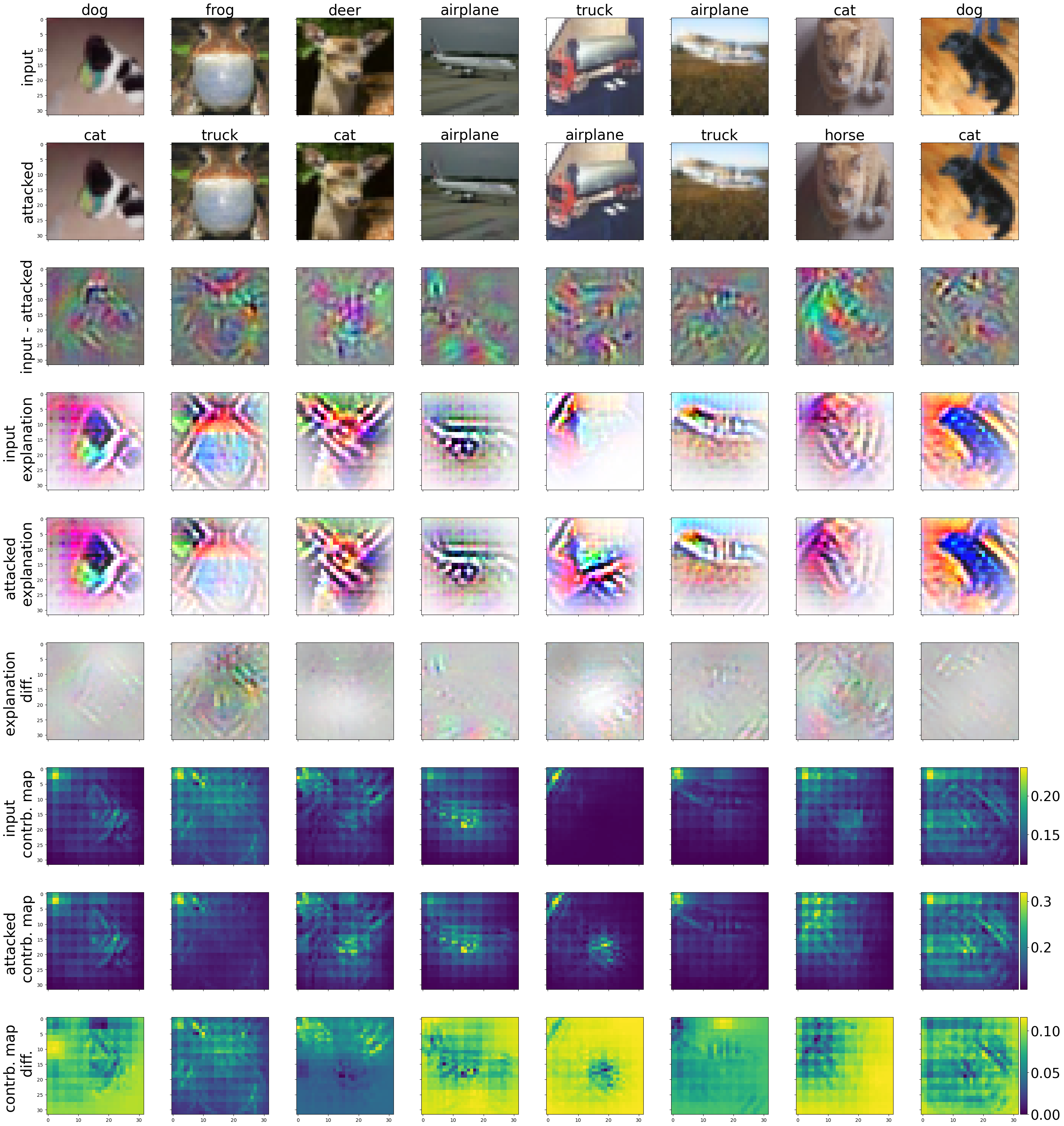
Fig. 4: Example of inputs to B-cos ResNet-50 attacked with \({\ell_2}\) PGD with 100 steps and \({\epsilon=0.5}\).

The \(\ell_2\) attack on the airplane image in Figure 4, column 4, was unsuccessful, and the corresponding attacked explanation remained largely unchanged. In contrast, the \(\ell_\infty\) attack in Figure 5 successfully misclassified the airplane image as a deer. This misclassification is reflected in the corresponding attacked explanation, which resembles a deer’s antlers, and in the reduced attention to the airplane engine in the attacked contribution map

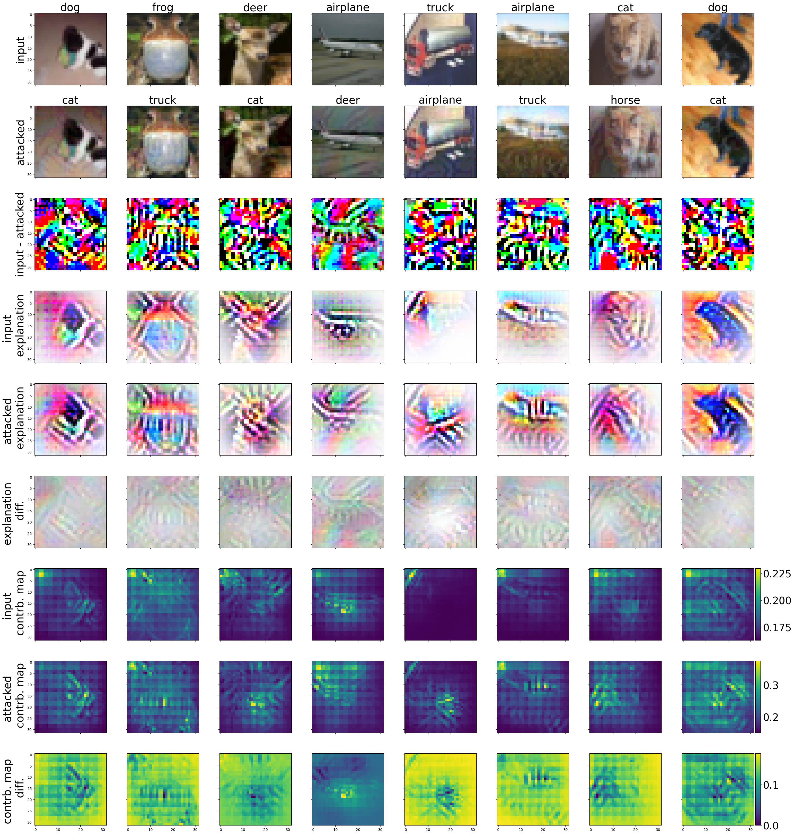
Fig. 5: Example of inputs to B-cos ResNet-50 attacked with \({\ell_\infty}\) PGD with 100 steps and \({\epsilon=8/255}\).

4.3 Adversarial Noise Comparison

Finally, I found it interesting to see the differences in adversarial noise produced by naturally, adversarially, and B-cos trained networks. Figure 6 shows a different set of inputs from the CIFAR10 test set, along with their corresponding adversarial noises generated by the four different models. The adversarially trained model was trained against \({\ell_2}\) PGD attacks with \({\epsilon=0.5}\). The adversarial attack depicted is an \({\ell_2}\) PGD attack with 100 steps and \({\epsilon=0.5}\). From the figure, it is evident that the adversarial noise generated by the standard model is more noisy and granular, while the adversarially trained model’s noise is more structural and input-aligned. The adversarial noise generated by the B-cos models appears to fall between the two.

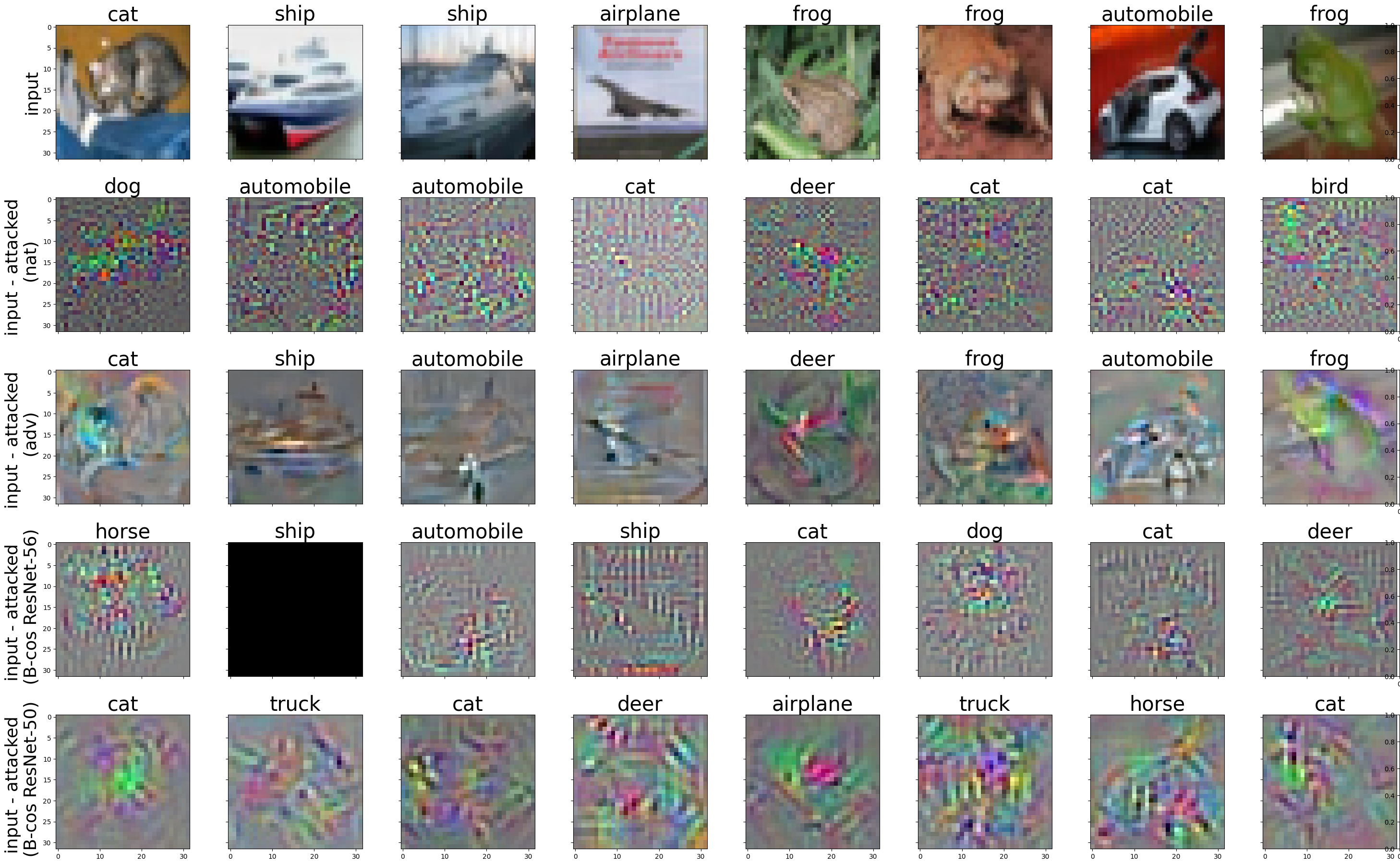
Fig. 6: Example of adversarial noise generated by \({\ell_2}\) PGD attack with 100 steps and \({\epsilon=0.5}\) for naturally, adversarially, and B-cos trained netwokrs.

5. Conclusion

While it was not rigorously investigated, as this was not the intent behind this post, B-cos models exhibited inherent robustness, especially against \(\ell_2\) PGD attacks, even surpassing adversarially trained models for the largest epsilon tested. In some instances, B-cos’ explanations and contribution maps shed light on why the model might have changed its decision. However, to draw firm conclusions on the robustness of B-cos models, a fairer and more comprehensive evaluation encompassing a variety of attacks is warranted. Additionally, it would be interesting to investigate the transferability of adversarial examples for B-cos models, the impact of B-cos hyperparameters (e.g., different B’s) on robustness, and whether adversarial training could further enhance their robustness and weight-input alignment.

6. References

1. Bohle, Moritz, Mario Fritz, and Bernt Schiele. “Convolutional dynamic alignment networks for interpretable classifications.” In Proceedings of the IEEE/CVF Conference on Computer Vision and Pattern Recognition, pp. 10029-10038. 2021.

2. Böhle, Moritz, Mario Fritz, and Bernt Schiele. “B-cos networks: Alignment is all we need for interpretability.” In Proceedings of the IEEE/CVF Conference on Computer Vision and Pattern Recognition, pp. 10329-10338. 2022.

3. Böhle, Moritz, Navdeeppal Singh, Mario Fritz, and Bernt Schiele. “B-cos Alignment for Inherently Interpretable CNNs and Vision Transformers.” arXiv preprint arXiv:2306.10898 (2023).

4. Logan Engstrom, , Andrew Ilyas, Hadi Salman, Shibani Santurkar, and Dimitris Tsipras. “Robustness (Python Library).” (2019).